Phase angle and flow pattern studies for inertance tube puise tube refrigerator Hatwar Rajeev1, Atrey M.D.1 1Mechanical Engineering Department, Indian Institute of Technology Bombay, Powai, Mumbai-400076 Abstract The phase angle between mass flow rate and pressure and the flow patterns in a Pulse Tube Refrigerator (PTR) are important factors which affect the performance of the refrigerator. Various modifications have been made to the PTR in order to reduce the phase angle and secondary flow, to increase the refrigeration effect. Secondary flow emerges due to the change in the cross-section and the direction of the flow. Flow straighteners and tapered pipes are used to avoid the formation of secondary flows. These secondary flows disturb the temperature profile in PTR, which in turn deteriorate the refrigeration effect. The present paper highlights the emergence of secondary flow in Inertance Tube Pulse Tube Refrigerator, especially near the cold end heat exchanger, and correlates it with the phase difference. The analysis further studies the effect of change in crosssection area on secondary flow and its effect on the performance of the PTR. The modelling of the ITPTR is done using commercial CFD software, FLUENT 6.2. From the analysis, it has been observed that, the phase difference between the mass flow rate and the pressure is responsible for the secondary flow. The duration of secondary flow per cycle is directly proportional to the phase difference. Hence reduction in the phase difference amounts to reduction in secondary flow. Top Keywords Inertance Tube Pulse Tube Refrigerator, CFD, Flow Pattern, Secondary Flows. Top |
INTRODUCTION The working of Pulse Tube Refrigerator (PTR) is fairly complex. Many theories have been proposed to explain the physical phenomena that take place in the PTR. One such theory is the Phasor analysis model which was proposed by Radebaugh [1], In this analysis it was concluded that the cooling capacity of the Orifice PTR (OPTR) is maximum when the phase difference between mass flow rate and pressure at the cold heat exchanger (HX) is minimum. Several modifications have been done to the basic PTR to reduce the phase angle and thereby improve the cooling capacity. Some of the important variations are OPTR [2], Double-inlet PTR [3] and ITPTR [4], |
The performance of the PTR also gets gets affected by the secondary flows [5]. Secondary flows disturb the temperature profile in PTR, which in turn deteriorate the refrigeration effect [6]. They emerge due to change in cross-section and direction of the flow. Flow straighteners and tapered pipes are used to avoid their formation [7, 8]. |
In the present work the flow pattern in the ITPTR has been analyzed by dividing the complete cycle of expansion and compression into different regions. The analysis is mainly focused to the key sections, near Cold HX and during flow reversals. On the basis of flow analysis the effect of phase angle and geometry on the performance has been studied. |
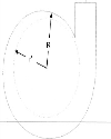
Top SIMULATION MODEL The dimensions of the ITPTR modelled here are taken from Cha et al. [9], The schematic of the ITPTR is shown in Fig. 1 and the dimensions of all the parts are mentioned in Table 1. |
ITPTR is modelled using commercial CFD software, FLUENT 6.2. Fluent requires a pre-processor for generating the geometry and the grid, for this purpose GAMBIT was used. |
Segregated solver is used for the modelling for its computational time efficiency. Implicit time integration scheme is used to get accurate results. In order to discretize the equations for density, momentum, energy and turbulence “second order upwind” scheme was used. PISO and PRESTO schemes were used for pressure velocity coupling and pressure, respectively, because of the porous media and transient flow. |
Fine mesh is used near the edges due to the possibility of large gradients. In order to model the piston motion in the compressor, a user defined function (UDF) is used. Dynamic layering method is used to take care of the deformation of the mesh near the piston which is in continuous motion. The amplitude and the frequency of the piston are 4.511 mm and 34 hz respectively. The motion of the piston is modelled as sinusoidal. |
The analysis of the ITPTR is done using a 2-dimensional axisymmetric model. Equations 1, 2 and 3 are the continuity, momentum and energy equations respectively [9,10]. |
The regenerator and the heat exchangers consist of steel and copper meshes respectively. To model these parts in FLUENT, porous media option is used. The mass, momentum and energy equations for these parts are given below [9, 10], |
The working fluid considered is Helium and has been modelled as an ideal gas. The thermodynamic properties of the gas and regenerator matrix material are considered at 300 K during this simulation. A laminar flow pattern is assumed in pulse tube and the inertance tube. Table 2 gives the boundary conditions used in the analysis. The convergence criteria (scaled residual) for mass and velocity are taken as 10−3, and 10−6 for the energy equation. |
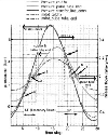
Top RESLTS AND DISCUSSION In the present analysis a complete cycle of expansion and compression has been divided into 30 time steps as shown in Fig. 2.At each time step, the flow pattern in the entire ITPTR has been obtained with the help of simulation. In order to carry out systematic study of the flow patterns in the pulse tube, the analysis has been divided into three parts: |
Flow patterns at the entrance of the pulse tube (near cold HX) Flow pattern at the end of the pulse tube (near hot HX) Flow pattern near the walls and at the corner of the pulse tube
In each of the three parts mentioned above, the analysis has been restricted to few key time steps where major changes in the flow pattern take place. The flow in the pulse tube is driven by the compressor. When the pressure in the compressor is higher than the pulse tube, the gas flows away from the compressor towards the pulse tube. But this process is not instantaneous as it takes some time for the flow to change its direction. It is during this time interval that secondary flows are observed. Further, the sudden changes in the cross-sectional area also cause secondary flow. |
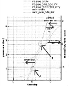
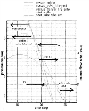
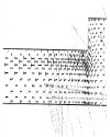
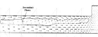
Flow patterns at the entrance of the pulse tube The compression and the expansion part of Fig. 2 have been highlighted in Fig. 3 and Fig. 5 respectively. It can be seen from Fig. 3 that during compression, the change in the direction of the mass flow rate (B) at the cold end HX occurs some time after the pressure in the compressor has risen above the pressure in the pulse tube (A). Similarly during expansion (Fig. 5) the direction of the mass flow rate (D) changes some time after the pressure in the compressor has gone below the pressure in the pulse tube. It should be noted here that the pressure is calculated at the centre of the cross section area. During these time intervals, while the direction of the flow catches up with the pressure, secondary flows are observed near the cold end heat HX as seen in Fig. 4 andFig:6. It can be seen from Fig. 4 thaf the direction of the flow near the wall has opposite direction then the flow near the axis. The swirl formation can be seen in Fig. 6. Flow pattern at the end of the pulse tube Similar phenomenon of time lag has been observed at the end of the pulse tube. In Fig. 2, points E and F represent the points of reversal of mass flow rate at the end of the pulse tube during compression and expansion respectively. It can be clearly seen from Fig. 2 that the points A and C come before points E and F respectively. Secondary flows are observed during this interval. Flow pattern at the corners and near the walls of the pulse tube Simulation results show that corners (sudden changes in the crosssection) play an important role in the development of secondary flows inside the pulse tube. In order to explain this, flow pattern near the hot end HX has been analyzed near points A and E, as shown in Fig. 7 and Fig. 8 respectively. Fig. 7 shows the portion of the pulse lube which is near the hot end HX at 5th time step. Before this time step the pressure in the pulse tube was higher than the pressure in the compressor due to which the flow is towards the left, in the pulse tube. At the 5th time step the pressure of pulse tube is still above that of the compressor, therefore the velocity is towards the left throughout the pulse tube. From Fig. 7 it can be seen that the velocity of the fluid is highest not at the centre (axis) but at a point which is approximately at a distance of 0.75*radius from the centre (“%” location). The reason for this kind of velocity is larger diameter of the hot end HX, as compared to the pulse tube. When the fluid from the hot end heat exchanger comes to the pulse tube, velocity of the fluid increases due to decrease in diameter (density does not change considerably). As the change of diameter is abrupt and the hot end HX is filled up with mesh, which gives high resistance to the flow, much of the increase in velocity is restricted near the wall. However due to resistance of the wall, the velocity of fluid just adjacent to the wall is very small. Due to all these factors the maximum velocity happens to be at “¾” location. Fig. 8 shows the flow pattern in the pulse tube when the mass flow rate is just about to reverse its direction. The encircled region is where the secondary flow can be seen. This is the same region where the velocity is the highest (“¾” location) few time steps earlier. Hence it is the last region to change its direction. Since it is an axisymetric figure, the secondary flow develops on both the sides of the axes. In case of gradual change in the cross-section, maximum velocity will occur at the centre of the pulse tube and this would lead to secondary flow at the centre thereby reducing the region of the secondary flow. It is to be noted that the secondary flow in the pulse tube is restricted to the portions highlighted in Fig. 2, and the secondary flows near the cold end HX is restricted to region between A, B and C, D. Phase difference is represented by Points B and E in Fig.2. Here point E represents the crossing of the mean pressure line by the pressure at the cold end HX. As the points B and E will come closer the distance between points A and B is going to reduce. Hence, it between the mass flow rate and the pressure reduces at the cold end HX, the time interval in which secondary flow occurs reduces. This implies that reduction in phase angle reduces the occurrence of secondary flow. Top CONCLUSION Commercial CFD code, FLUENT 6.2, is used to model ITPTR. An attempt is made to analyze the effects of phase angle on the secondary flow using flow analysis as a tool. From the analysis, it is clear that, the phase difference between the mass flow rate and the pressure is responsible for secondary flow. The duration of secondary flow per cycle is directly proportional to the phase difference. Hence, the reduction in phase difference amounts to the reduction in secondary flow. Further, the flow analysis also helps to understand how sudden changes in the cross section area contribute to the emergence of secondary flow inside the pulse tube. |
Top Nomenclature Figures | Figure 1.: Schematic of the ITPTR
|  | |
| | Figure 2.: Variation of pressure with time at 1) compressor, 2) cold end HX and 3) pulse tube end; and variation of mass flow rate with time at 1) cold end HX and 2) pulse tube end
|  | |
| | Figure 3.: Compression phase
|  | |
| | Figure 4.: Velocity vectors at the entrance of the pulse tube at 7th time step
|  | |
| | Figure 5.: Expansion phase
|  | |
| | Figure 6.: Velocity vectors at the entrance of the pulse tube at 21st time step
|  | |
| | Figure 7.: Velocity vectors in right half of the pulse tube along with hot HX, at 5th time step
|  | |
| | Figure 8.: Velocity vectors in right half of the pulse tube at 9th time step
|  | |
|
Tables | Table 1: Dimensions of various parts of ITPTR
| | Components | Radius(mm) | Length(mm) | | A (Compressor) | 9.54 | 7.5 | | B (Transfer line) | 1.55 | 101 | | C (After cooler) | 4 | 20 | | D (Regenerator) | 4 | 25 | | E (Cold end HX) | 3 | 5.7 | | F (Pulse Tube) | 2.5 | 30 | | G (Hot end HX) | 4 | 10 | | H (Inertance Tube) | 0.425 | 684 | | 1 (Reservoir) | 13 | 130 |
| | | Table 2: Boundary conditions
| | Components | | | Aftercooler wall temperature | 293 K | | Cold end HX condition | Adiabatic | | Warm end HX temperature | 293 K |
| | :
| | inertial drag coefficient tensor (m−1) | | h | enthalpy (J/kg) | | j | superficial velocity | | k | thermal conductivity (W/m K) | | P | pressure (N/m2) | | T | temperature (K) | | t | time (s) | | V | intrinsic velocity (m/s) | | Greek letters | | permeability tensors (m2) | | ε | porosity | | μ | absolute viscosity (kg/m s) | | ρ | density (kg/m3) | | stress tensor (N/m2) | | Subscripts | | f | fluid | | r | radial coordinate | | s | solid | | X | axial coordinate |
| |
|